The purpose of this project is to deburr the Airplane Gear Teeth (shown in the pic. on the left) with the industrial robot. Even though the desired deburring path on the gear teeth is irregular, it is composed with basic configurations of circles and rectangles. Therefore, before actually deburring the gear teeth, we researched on deburring circular and rectangular aluminum blocks first to evaluate the methods and performances.
As the program goes, we found that there will be three iterations in general: Iteration One: Deburr circlular and rectangular aluminum block edges precisely; Iteration Two: Chamfer circlular and rectangular aluminum block edges; Iteration Three: Deburr one tooth of airplane gears.
Iteration One: Deburr circlular and rectangular aluminum block edges precisely
1. Circle
video: duration: 00:00:04
As shown in the video, the end effector deburrs the edge of the cylinder along a precise circular path with the hard brush verticlely. This step proved that a circular trajectory design is feasible.
2. Rectangle
video: duration: 00:00:06
As shown in the video, the end effector deburrs the edge of the rectangular block along a precise linear path with the hard brush verticlely. This step proved that a linear trajectory design is feasible. However, to avoid the corner collisions, I had the robot stop at every corner of the block, which resulted in a inconsistency of the feedrate. This problem will be taken care in the Iteration Two after I add more features upon this method.
Iteration Two: Chamfer circlular and rectangular aluminum block edges
In the Iteration Two, I updated two things: Firstly, I adjusted the end effector tool angle so that it would create a chamfer on the parts when deburring; Secondly, I changed the deburring path of the rectangle so that the feedrate would be consistent while still being able to avoid corner collisions.
1. Circle
video: duration: 00:00:08
In the circular path design, besides changing tool angles, I also wrote a simple MatLab programs to determine the center point and the radius of a circle given three points on the edge. The necessity of doing that is because in the actual implementation of the parts onto the table, the position of the part can be slightly off as there are tolerances on both mounting hole and screw bolt. Therefore, whith this code, I just need to jog the tip of the end effector at three different points along the cylinder edge, and I would know the center point and the radius of the cylinder part. The code is shown as below:
clear
clc

% User input data
promptx1='x1= ';
x1=input(promptx1);
prompty1='y1= ';
y1=input(prompty1);
promptx2='x2= ';
x2=input(promptx2);
prompty2='y2= ';
y2=input(prompty2);
promptx3='x3= ';
x3=input(promptx3);
prompty3='y3= ';
y3=input(prompty3);

% calculate center X & Y and redius R
MX1=(x1+x2)/2; MY1=(y1+y2)/2; G1=(y2-y1)/(x2-x1);
MX2=(x2+x3)/2; MY2=(y2+y3)/2; G2=(y3-y2)/(x3-x2);
A=[1/G1 1;1/G2 1];
C=[MY1+MX1/G1;MY2+MX2/G2];
B=A\C;
X=B(1); Y=B(2);
R=sqrt((x1-X)^2+(y1-Y)^2);

% print
fprintf('The center of the circle is (%8.5f, %8.5f),\nThe redius of the circle is %8.5f mm\n',X,Y,R);
2. Rectangle
video: duration: 00:00:13
In this iteration for rectangle, besides changing the end effector tool orientation, I also edited the deburring path of the rectangle. As shown in the picture on the right, at each corner, I added an extra detour so that the robot did not have to stop to avoid the corner collisions.
Iteration Three: Deburr one tooth of airplane gears
This week we will deburr one of the gear teeth, and the results will be updated soon.
December, 2014 ~ May, 2016
Project B:
Navigation Mappings
Human-Robot Interaction Lab, Oregon State University
Advisor: Cindy Grimm
Maps — specifically floor plans — are useful for a variety of tasks from arranging furniture to designating conceptual or functional spaces (e.g., kitchen, walkway). We present a simple algorithm for quickly laying a floor plan (or other conceptual map) onto a SLAM map, creating a one- to-one mapping between them. Our goal was to enable using a floor plan (or other hand-drawn or annotated map) in robotic applications instead of the typical SLAM map created by the robot. We look at two use cases, specifying “no-go” regions within a room and locating objects within a scanned room. Although a user study showed no statistical difference between the two types of maps in terms of performance on this spatial memory task, we argue that floor plans are closer to the mental maps people would naturally draw to characterize spaces.
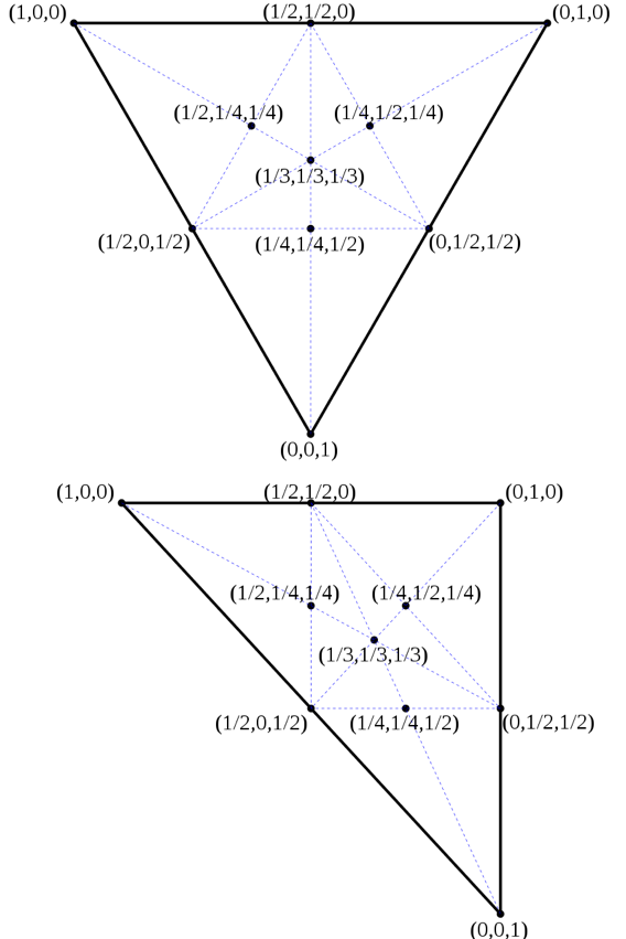
As shown in the video, if two maps (for the same room) overlap, they would not exactly match each other. To correlate corresponding reagions between two maps, we apply the "Barycentric Coordination Algorithm" (shown in picture at left): Two maps are dissolved into same amount of tiny triangles, and we match the barycenters of two same-located triangles between maps.
The specific algorithem is illustrated in the python code below:
As the result, we have presented a simple technique for mapping a hand-drawn sketch or floor plan to a SLAM map, and conducted a user study looking at the effectiveness of the floor plan over a SLAM map for a spatial memory task. There was no statistically significant difference in the average performance, however there was a slight difference in the kinds of errors the participants made. To gain a fully understanding of the research, please refer to the paper we published on ICSR (International Conference on Social Robotics) 2016:
Or, as an alternative, you could briefly go through the project by watching my presentation on ICSR 2016:
Manufacturing Process Control Laboratory, Oregon State University
Advisor: Burak Sencer
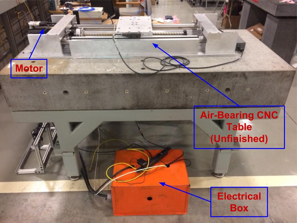
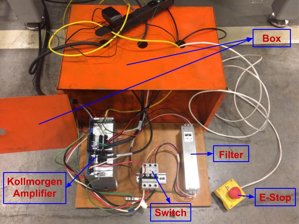
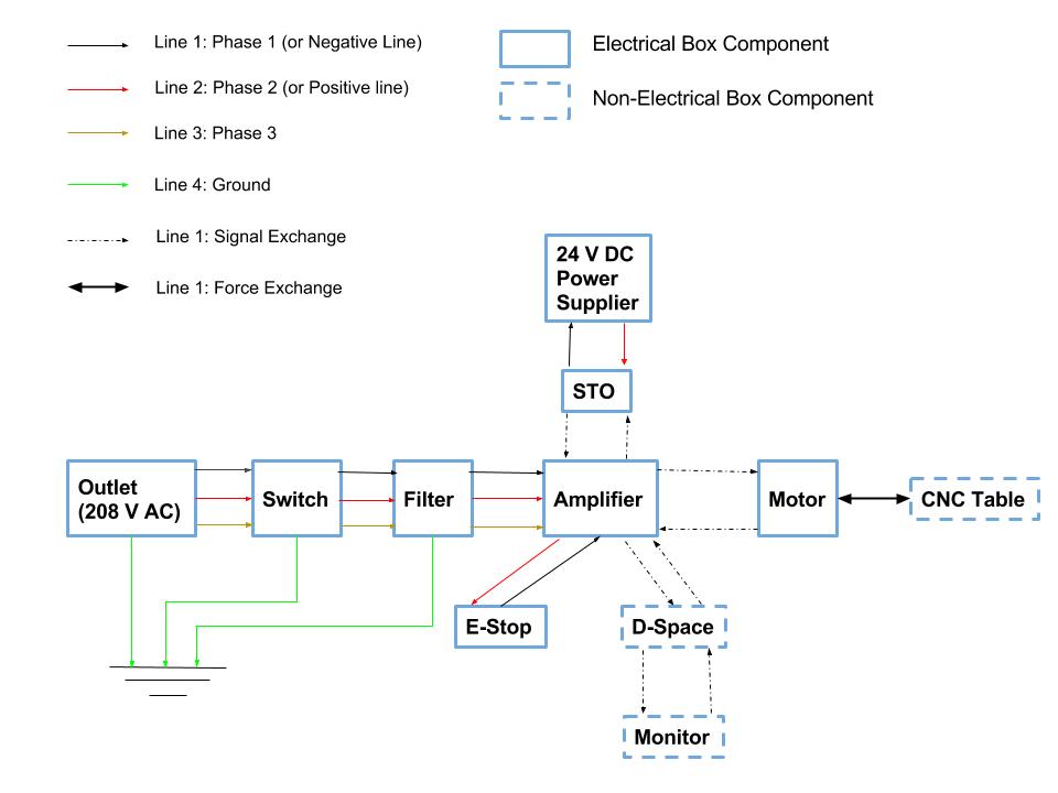
The Electrical Box for CNC Machine is to provide purified electricities and programmable signals for the motor, which drives the CNC Table and guarantees precise motions. The electrical box is composed of: Switch, Filter, Amplifier, E-Stop, Motor and Metal box. The diagram below illustrates the connections between those components:
The functionalities of each component are listed below:
1. Three-Phase Power Supply: Three-phase electric power supply is used to support the three-phase induction motor. How it works is three conductors each carry an alternating current of the same frequency and voltage amplitude relative to a common reference but with a phase difference of one third the period. In comparison with single-phase power supply, three-phase power supply can carry heavier load, and it is also more ecnomically efficient.
2. Switch: Switch is out-of-box and is used to manually turn on and off the system. As the result, I selected a 3 Poles-Toggle Style, DIN-Rail Mount AC Equipment Circuit Breaker.
3. Filter: Electrical filter is out-of-box and is used to filter out the noises in electricities. In this scenario, I chose a 488/277 VAC, 16 A 1-Stage filter from the Schaffner Company.
4. E-Stop: Emergency Stop Button is out-of-box and is used to immediately cut power with a single push in emergent situations.
5. 24 V DC Power Supplier: 24 V DC Power Supplier, also called AC-to-DC transformer, is out-of-box and is used to translate 120V AC power into 24V DC power. In this appication, the 24V DC power is used to power the Safe Torque Off (STO) feature.
6. STO: Safe Torque Off (STO) is a restart lock safety feature that is embedded inside of Amplifier. It is used to protect personnel by preventing an unintentional system restart.
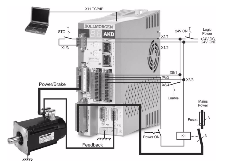
7. Amplifier: Amplifier is the "CPU" of the electrical box, and I selected the Kollmorgen AKD Amplifier in the project. As illustrated in the Diagram above, electricities coming out of the filter goes through the amplifer to power on the motor. At the same time, the amplifier is tuned through its software (Kollmorgen Workbench) to determine the inertias and friction factors of the free motor. In addition, the E-Stop and STO will cut the power of the amplifier first whenever a emergency occurs. Also, the D-Space equipment is connect with the Amplifiers to exchange control signals with it. Below is the minimum wiring for the amplifier:
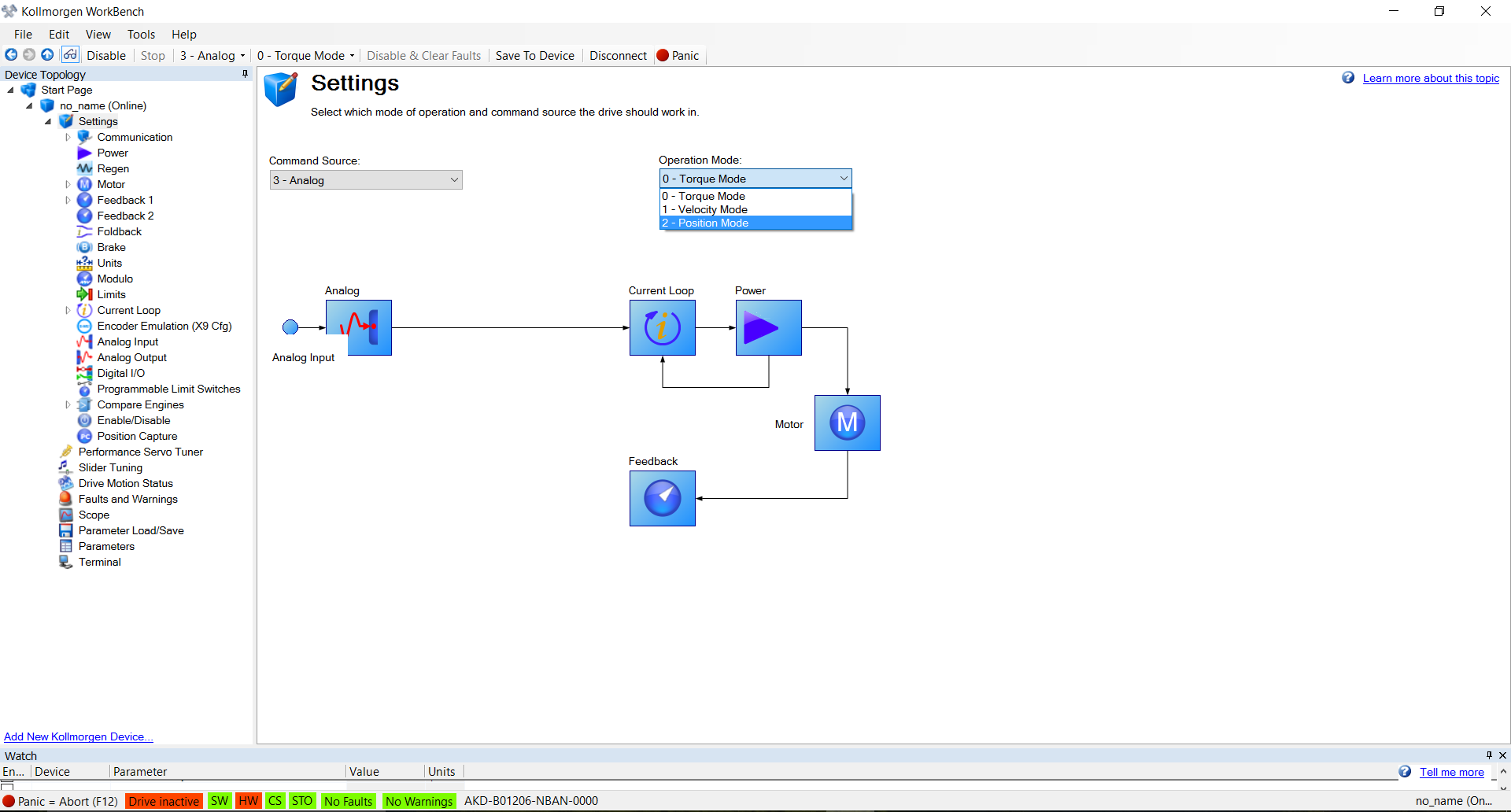
8. Motor Tuning: Workbench is a tuning software comes with the Kollmorgan Amplifier. It is used to adjust the motor to yield its optimal performance. Below is the main page of the software interface, as shown in the screenshot, the system is tuned with position/current loop.
Here is the tuning procedure: Firstly, as shown in the Amplifier Wiring Diagram, an ethernet cable connects the PC and the X11 port of the amplifier, and the IP address of the amplifier is configured properly on the same subnet as the controll. Secondly, a signal generator is connected to the analog input port (X7), and an oscilloscope is connected to the analog output port (X8). Lastly, adjust the analog input and output scale parameters in the software to make sure that the performance of motor and the outcome signal on the oscilloscope match the signal input.
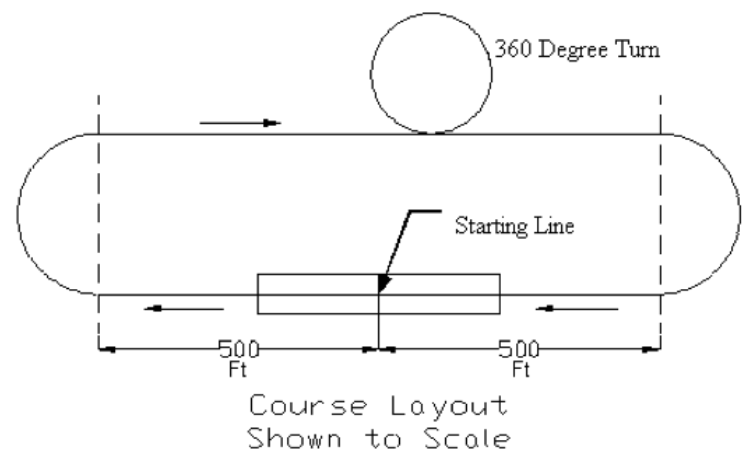
This project was designed to participate in the 2016-2017 American Institute of Aeronautics and Astronautics (AIAA) Design/Build/Fly (DBF) competition in Tucson, Arizona. This year’s Design/Build/Fly competition required teams to build an aircraft capable of being stowed in a small launch tube, although the aircraft did not need to launch from the tube. The payload consisted of regulation size hockey pucks (3'' dia X 1 in thickness, 5.5-6 oz), and payload requirements changed for each mission ranging from no payload to as many pucks as the team wished. All aerial missions was flown on the course layout shown in Figure on the left. The team was divided into aerodynamics, structure, control/propulsion and material/manufacturing subteams, with each team being responsible on their own topic while smoothly cooperating with other subteams at each UAV design stage.
Wing Developement
A successful wing design was one of the importance, and the design process was iterative. a. Materials:
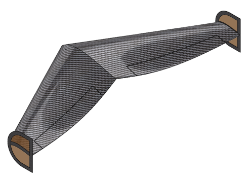
We firstly selected T800 Plain Weave Carbon Fiber as wing material, because it is lightweight, flexible, moldable yet strong. b. Aerodynamics:
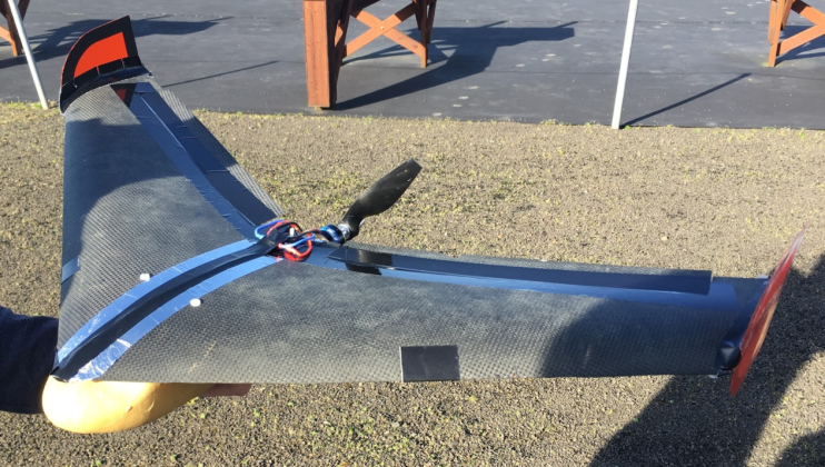
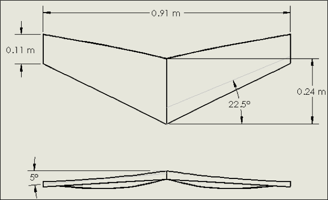
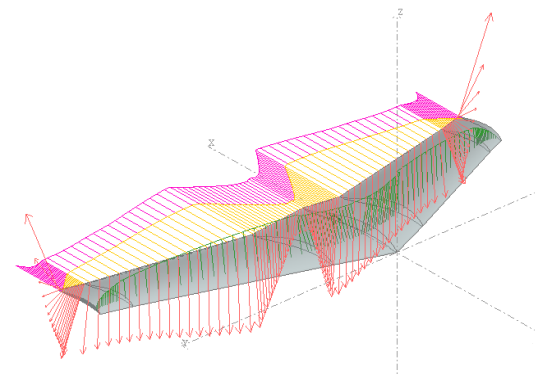
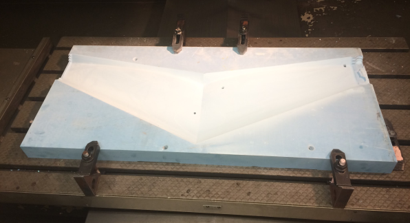
THen, we designed the wing geometry and slected the airfoil based on the required weight, aspect ratio and speed. As the result, our design had a maximum airfoil coefficeint of lifting (CLmax) as 1.65, and the maximum wing lift-drag coefficient as 1.42, which combined could guarantee a sufficient lift, basic stability during flight and manageable landing speed. Figures below show the final geometry and airfoil design: c. Structure: In the stability test stages, we found the flights were highly vulnerable to the disturbance of wind. Therefore, as shown in the figure on the right. we added winglets at the tips of the wing, to serve the purpose of adding more drag on the low pressure side of the wing. As the results, the flights did become way more stable then before. d. Control: The challenge of control surface design was to accommodate the folding wing design. As the results, we cut out the control surface from the wing, and then reattached it. The span of the control surface was 300 mm and it occupied 20% of the chord. e. Manufacture: To mold the wing, the team selected machinable high-density high-temperature (HDHT) toolboard. This material is quickly and easily machined by CNC to near-exact specifications, as shown in the figure below on the left. The final step before wing manufacturing was creating a flat pattern. The pattern was optimized to increase torsional stiffness along the span of the wing while still allowing for the tight bend radius required for storage in the tube. Using the pattern in figure below on the right, four pieces of carbon fiber were cut out and laid up on the mold. The wing and mold were then enclosed in a vacuum bag and cured for 8 hours at 250° F. After cooling back to room temperature, the wing was separated from the mold, any excess resin was removed, and the pressure side of the wing was finely sanded to reduce drag.
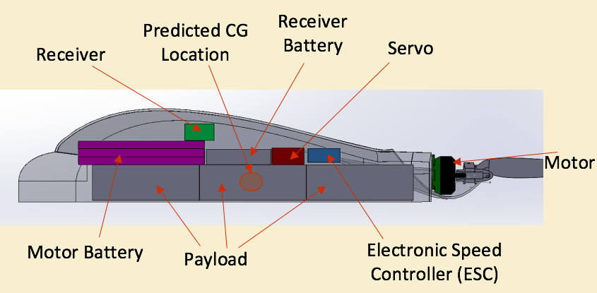
Main Body
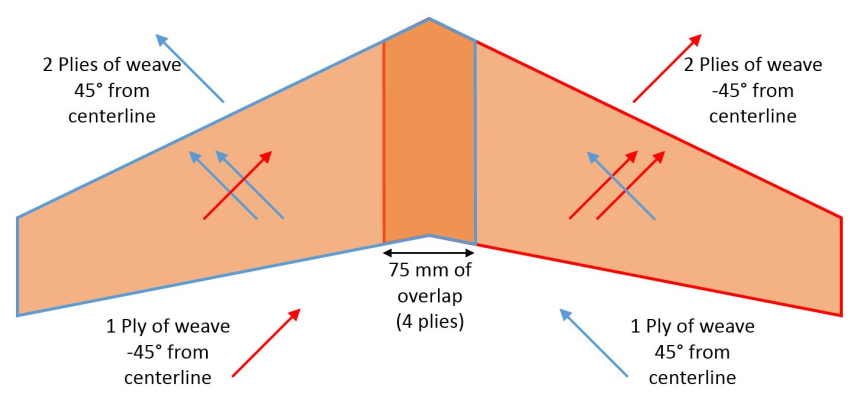
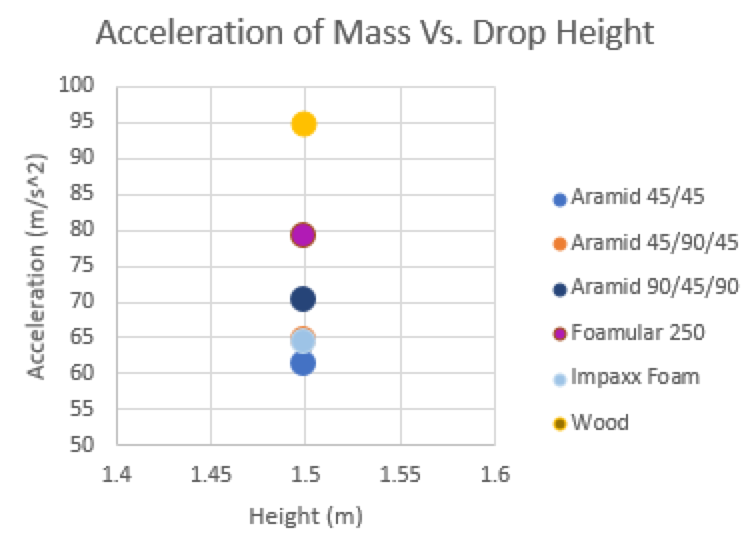
Main body housed payload, propulsion system and RC system, and it is also where the wing was mounted at. It was important for its aerodynamic shape to be able to handle low drag. a. Design Solution: Too minimize the aerodynamic drag and wetted surface area, NACA0027 shape was slected as main body shape. b. Main Body Structure: As shown in the diagram below, the motor mounted in the aft section of the UAV created a moment about the centerline of the motor. This torque was transmitted through four stainless steel fasteners that passed through the rigid 1/16” plywood motor bulkhead. The plywood distributed the load through the entire UAV. Also, the main body resisted the weight of the motor bulkhead, payload and electronics through the implementation of hoop and longitudinal stiffenered. These stiffeners were composed of Divinycell foam sandwiched between two ±45° aramid fabric plies. c. Nose Cone Structure: According to the result of nose dropping test, as shown in the figure on the right, the aramid fabric nose cone was designed to deform and absorb much of the impact energy to protect components within the main body in the event of a high impact, nose-down crash.
Propulsion System
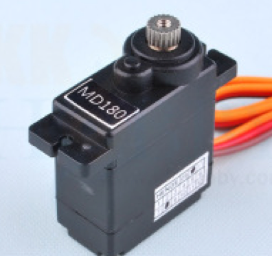
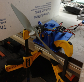
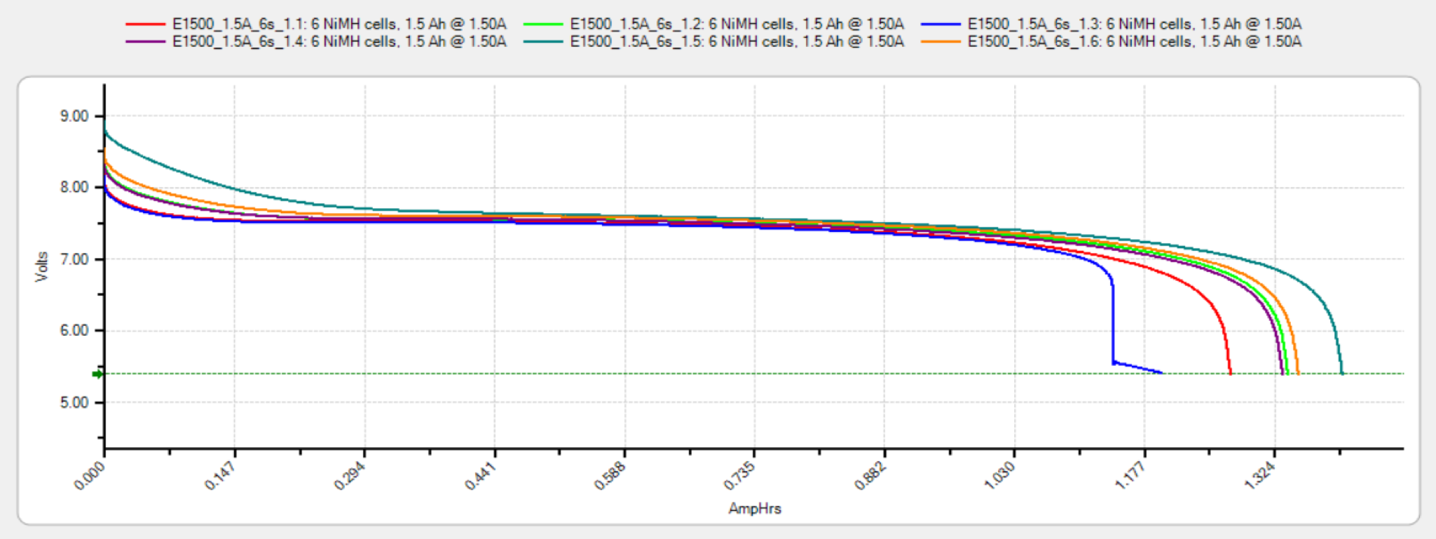
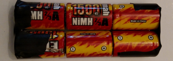
All of the propulsion components were out-of-box. Propulsion team's responsibility was to select the proper components and test their properties to match the requirements of flight. a. Receiver/Transmitter Selection: The receiver chosen was the Spektrum AR6210 6-channel receiver. It featureed a failsafe system to comply with competition safety regulations and was lightweight. The transmitter used was a Spektrum 20-model memory board transmitter. b. Servo Selection and Integration: Two servos were used to actuate the left and right elevon control surfaces and were housed within the payload tray. Small cut-out windows on the main body allowed for the servo arms to extend outside and actuate the elevons using aluminum rods. Housing the servos within the main body reduced drag and allowed the wing to feasibly wrap around in storage. Control surfaces were modelled in XFLR5 at maximum deflection angles to analyze hinge moments and determine the servo torque required. The servo selected for each elevon was the TowerPro SG90 because it is lightweight and provides sufficient torque. c. Motor and Propeller Selection: The motor selected was the Cobra C-2204/32 brushless motor for its minimal weight and sufficient power generation. The propeller selected was an 8x4.5 folding propeller, which provided sufficient thrust to the UAV when housing a full payload yet allows the UAV to store inside a compact tube. Various motor and propeller combinations were tested to find the most lightweight option capable of meeting thrust requirements. The electronic speed controller (ESC) selected for the motor was the Cobra 11A. Pictures below shows the trust test (left) and the result of battery-draw test (right). The x axis represents for AmpHrs, whilte the y axis represents for Volts. d. Battery Selection: A six cell Elite 1500 NiMH battery pack was selected to power the propulsion system, as shown in the picture on the right. Battery selection was based off previous OSU DBF team’s testing. Determining the size of the battery pack was based on mission simulation calculations and verified in flight tests.
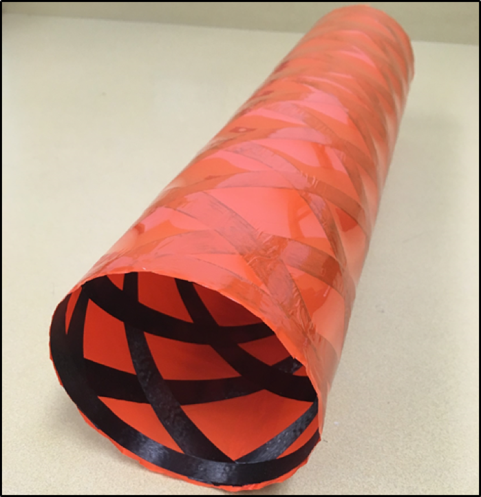
Tube Design
The tube experienced hoop stress when the wing was wrapped around the fuselage as well as longitudinal stress from impact loads during drop tests on each of the tube faces. The carbon fiber lattice structure was rigid enough to statically keep its shape yet tough enough to deform during a drop and return to its original shape. The plastic Mylar provided a constant compression force on the tube to resist the hoop stress from the folded wing as well as moisture protection.
Flight test performance
The whole project lasted for around 8 months, and ended up with the fifth place in this year's competition. This video shows one of our successful flights:
Energy Innovation Laboratory, Oregon State University
Advisor: Hailei Wang
The purpose of this project is to design an ice battery that stores the electrical energy at night and releases the stored energy at day time. Even through this method does not necessarily save more energy than AC, it does save money. As shown in the figure on the right, in some states (like california), the electricity fee at day time is four times of the electricity fee at night.
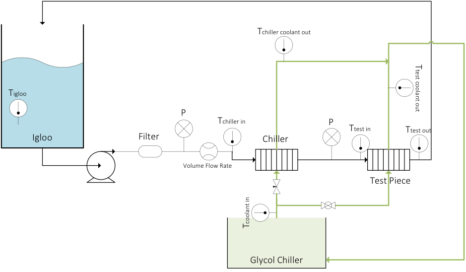
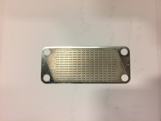
As shown in the diagram above, the designed system is composed of two cycles: Water cycle (balck line) and refrigerant cycle (green line). The refrigerant cycle runs extremely cooled refrigerant, so that it could exchange energy with pure water at Chiller and Test Piece. Both Chiller and Test Piece are heat exchangers, with the micro-channel design shown on the left. The purpose of Chiller is to cool the water down to near-zero degree, and the Test Piece is used to further cool down the liquid water into super-cooled water. Since super-cooled water is meta-stable, it would change from liquid to ice immedrately after it gets out of the tube and hit into the tank. In this way, the energy is stored in the form of ice. At day time, the ice-liquid mixture in the tank can be run over the system that needs to be cooled.
In general, the research had four stages: Coated/Uncoated test, PTFE stability test, PTFE low-temperature test and Desalination test.
Experimental System Set-up
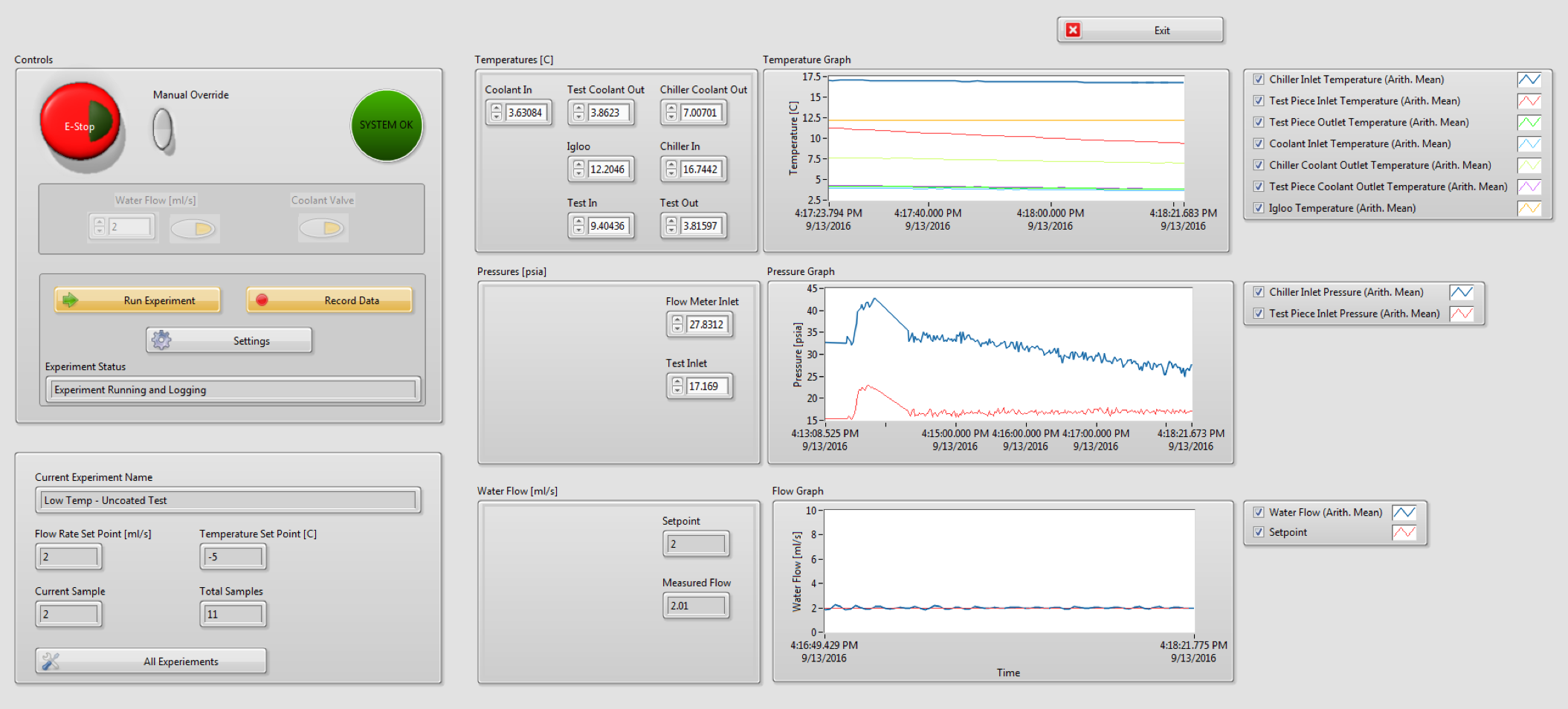
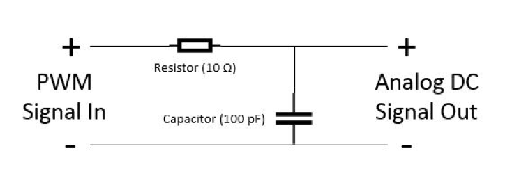
To test the design properties with the system, a lot of data needs to be collected. For example, in 100 experiments, how long is the average running time? At which part does the water freeze frequently? What was the lowest super-cooled temperature within those experiments? etc. Therefore, we introduced a LabVIEW-controlled automatic system into the cycles: a. LabVIEW: LabVIEW is used to automate the cycles. When the system runs without freezing, the signals collected by sensors would be transferred into analog data in national instrument (NI) equipments, then the labview processes those data and compare with the previous data to determine the system's status. At the same time, those data is recorded in the Microsoft Excel for researchers to analyze later. Whenever the LabVIEW detects a sharp decrease on flow rate, the system would report freezing and then shut down the solenoid valve in refrigerant cycle. At the same time, pump would continue to work so that the water cycle could restore sooner. Whenever the flowrate increases till the setpoint, the selonoid velve opens and the second experiment starts. The picture below shows the LabVIEW user interface. b. FlowMeter: Flowmeter is a key part in the hardware-software interaction, for the signals it releases determine if the cycles freeze or thaw. In the real application, anti-corrosion flowmeters that directly releases analog data can be as expensive as $10,000, and the flowmeter we got is Adafruit Flow Meter, which worths $20 and releases Pulse Width Modulation (PWM) signals. However, the NI Analog Input block reads only anaog data. As a result, a RC circuit that transfer the PWM signal to analog signal was designed, as shown in the diagram on the right. An Arduino Board was used for establishing the RC circuit, and the program part is attached at the end of the project in case for the further reference.
Coated/Uncoated test
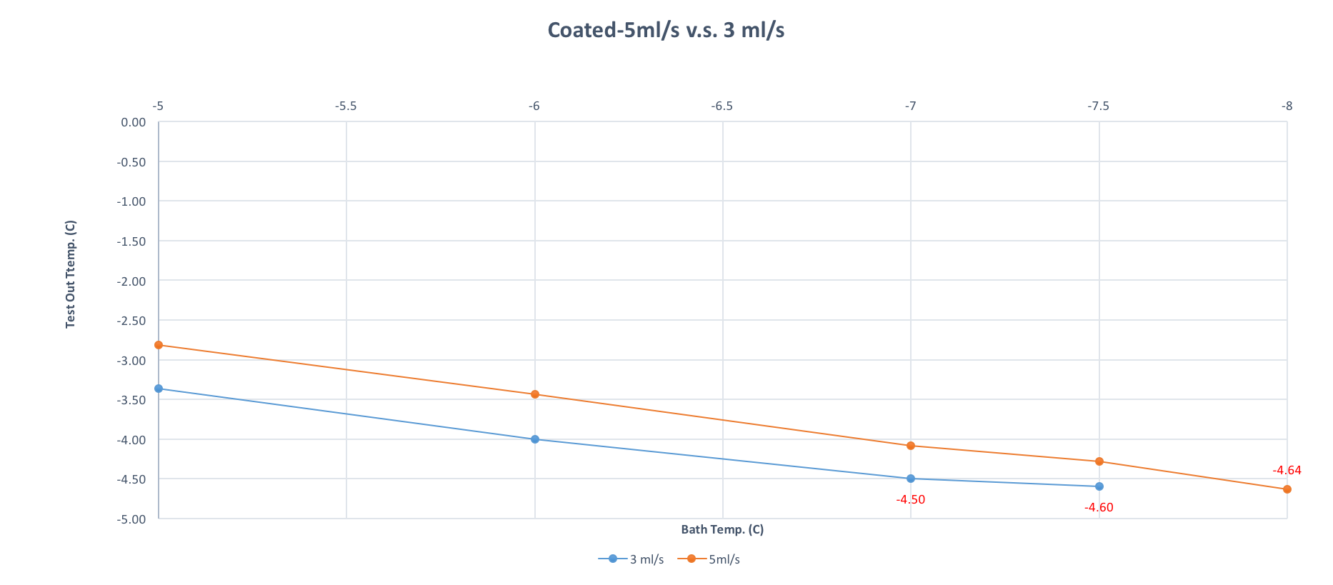
As the super-cooled ID water is meta stable, it is very possible that it freezes at its lowerst temperature, which is the Test Piece Outlet, with little disturbance. Therefore, it came to our minds that having the heat exchanger sheets' surfaces being coated may increase the contact angle of the water inside of the heat exchanger, so that the super-cooled water becomes more stable. We tried three coating materials: Fluorocarbon coating, Nano-florocarbon coating and Organosilane coating. As the results, it proved that the Fluorocarbon coating lasts longest. With the Fluorocarbon coating as the selected coating material, we measured and compared the Test Out Temperatures of coated system and uncoated system. The lower the outlet temperaturem, the more stable of the system. As the result, we found the coated system outperforms the uncoated one. In the future experiments, we all apply the coated system.
PTFE stability & low-temperature test
PTFE, also called Teflon, is the abbreviation of Fluorocarbon. With this material being coated in the system, we conducted the stability & low-temperature tests: measure the Test Piece Outlet temperature while decreasing the refrigerant temperature until the system freezes. Then, repeat the same procedure with a different flow rate. Below attached is one of typical results:
As shown in the graph, the smaller the flowrate, the more stable the system is. Also, we found that the system would freeze within 30 mins if the flowrate goes over 5 ml/s.
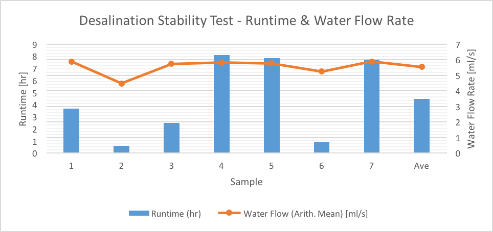
Desalination test
The purpose of the desalination test is to test the effects of applying this technology into ocean water: ID water is changed into simulated ocean water. As the freezing point of salt water is 3olower than ID water, it was expected the salt water is more stable.
As the result, it did prove that the system is more stable, for its runnng hours can be as long as 8 hours, as shown in the chart below, while the ID water could last for only around 3 hours with the same flowrate.
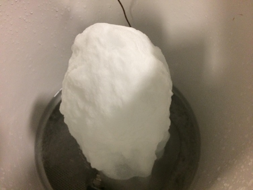
In addition, we unexpectedly found that this technology can desalinate the ocean water. As shown in picture at right, after around 10 hours' gravity dry, the salinity of the ice can be as low as only 1%. Therefore, this technology provides a possible way of desalinating ocean water in a low-energy way. However, the salt water corrodes the system severely, and it is still a challenge in front our team to put this research idea into business product.
Reference: Arduino Code - Converting PWM Signal into Analog Signal
#include "LiquidCrystal.h"
LiquidCrystal lcd(7, 8, 9, 10, 11, 12);

// which pin to use for reading the sensor? can use any pin!
#define FLOWSENSORPIN 2

int VoutPin = 9;
unsigned long previousMillis = 0;
const long interval = 1000;

//int analogPin = 3;
float liters;
int val;
float rate[10];

// count how many pulses!
volatile uint16_t pulses = 0;
// track the state of the pulse pin
volatile uint8_t lastflowpinstate;
// you can try to keep time of how long it is between pulses
volatile uint32_t lastflowratetimer = 0;
// and use that to calculate a flow rate
volatile float flowrate;
// Interrupt is called once a millisecond, looks for any pulses from the sensor!
SIGNAL(TIMER0_COMPA_vect) {
  uint8_t x = digitalRead(FLOWSENSORPIN);

  if (x == lastflowpinstate) {
    lastflowratetimer++;
    return; // nothing changed!
  }

  if (x == HIGH) {
    //low to high transition!
    pulses++;
  }
  lastflowpinstate = x;
  flowrate = 200.0;
  flowrate /= lastflowratetimer;  // in hertz
  lastflowratetimer = 0;
}

void useInterrupt(boolean v) {
  if (v) {
    // Timer0 is already used for millis() - we'll just interrupt somewhere
    // in the middle and call the "Compare A" function above
    OCR0A = 0xAF;
    TIMSK0 |= _BV(OCIE0A);
  } else {
    // do not call the interrupt function COMPA anymore
    TIMSK0 &= ~_BV(OCIE0A);
  }
}

void setup() {
  Serial.begin(9600);
  Serial.print("Flow sensor test!");
  lcd.begin(16, 2);

  pinMode(FLOWSENSORPIN, INPUT);
  digitalWrite(FLOWSENSORPIN, HIGH);
  lastflowpinstate = digitalRead(FLOWSENSORPIN);
  useInterrupt(true);

  pinMode(VoutPin, OUTPUT);
}

void loop()                     // run over and over again
{
  //lcd.print(flowrate);
  //lcd.print(flowrate);
  //Serial.print("Freq: "); Serial.print(flowrate);

  while (liters != -100) {

    unsigned long currentMillis = millis();
    if (currentMillis - previousMillis >= interval) {
      previousMillis = currentMillis;

      lcd.setCursor(0, 0);
      lcd.print("Pulses:"); lcd.print(pulses, DEC); lcd.print(" Hz: \n");
      Serial.print(" Pulses: "); Serial.print(pulses, DEC); Serial.print("\n");
      liters = pulses;
      liters /= 7.5;
      liters = 1.5354 * liters; // Calibration
      pulses = 0;

      // delay(20);


      rate[9] = rate[8];
      rate[8] = rate[7];
      rate[7] = rate[6];
      rate[6] = rate[5];
      rate[5] = rate[4];
      rate[4] = rate[3];
      rate[3] = rate[2];
      rate[2] = rate[1];
      rate[1] = rate[0];
      rate[0] = liters;
      float AveRate = (rate[9] + rate[8] + rate[7] + rate[6] + rate[5] + rate[4] + rate[3] + rate[2] + rate[1] + rate[0]) / 10;
      //val = analogRead(analogPin);
      //val *= (255/1023);
      val = (AveRate / 0.90) * 225;
      analogWrite(VoutPin, val);
      Serial.print(" Flow rate: "); Serial.print(liters); Serial.print(" Liters/min \n");
      Serial.print(" rate[9]: "); Serial.print(rate[9]); Serial.print(" Liters/min \n");
      Serial.print(" rate[8]: "); Serial.print(rate[8]); Serial.print(" Liters/min \n");
      Serial.print(" rate[7]: "); Serial.print(rate[7]); Serial.print(" Liters/min \n");
      Serial.print(" rate[6]: "); Serial.print(rate[6]); Serial.print(" Liters/min \n");
      Serial.print(" rate[5]: "); Serial.print(rate[5]); Serial.print(" Liters/min \n");
      Serial.print(" rate[4]: "); Serial.print(rate[4]); Serial.print(" Liters/min \n");
      Serial.print(" rate[3]: "); Serial.print(rate[3]); Serial.print(" Liters/min \n");
      Serial.print(" rate[2]: "); Serial.print(rate[2]); Serial.print(" Liters/min \n");
      Serial.print(" rate[1]: "); Serial.print(rate[1]); Serial.print(" Liters/min \n");
      Serial.print(" rate[0]: "); Serial.print(rate[0]); Serial.print(" Liters/min \n");
      Serial.print(" AveRate: "); Serial.print(AveRate); Serial.print(" Liters/min \n");
      Serial.print(" Output: "); Serial.println(val); Serial.print("\n");
    }
  }

}
Spring, 2017
Graduate Course Project:
NC Part Programming and Machining
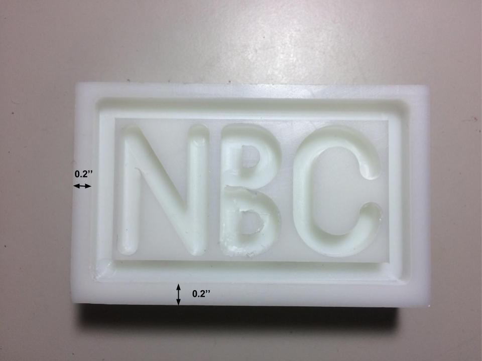
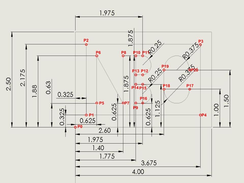
The purpose of this project is to design and machine a part on a CNC machine. As shown in the picture above, a blank rectangular block with specific dimensions was given, and I was required to design my part with the given dimensions and leave 0.2 inch from the edges of the part for fixturing and safety. The cutting tool has a diameter of D=1/4 inch and it is a 4 flute solid end-mill. The maximum federate of X and Y axis is 12 inch/min, and Z 2 inch/min. The spindle speed is selected to be S=750 rpm, and the cutting depth was 1/2 inch. The design includes three steps: Design geometry with the SolidWorks, define and gain the locations of points and generate NC codes.
Design with the SolidWorks
To design an appropriate part, I firstly sketched a rough draft and made sure that the diameter of drill bit was calculated in, so that the letters would not overlap with each other while being machined. Then, I transferred the sketch into a precise SolidWorks drawing, as shown below:
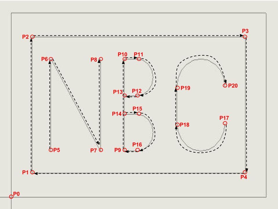
Define and gain the locations of points
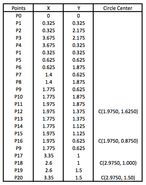
After the SolidWorks design, 20 pints was defined in sequence of machining, as shown in figure below:
In addition, the location of those 20 ponts in relative to the origin are listed in table below (G-code table):
Generate NC codes
Based on the G-code table, a NC code was generated accordingly:
Paper Repeat: Exponential Trajectory Generation for Point to Point Motions
Paper: Exponential Trajectory Generation for Point to Point Motion
Author: Z. Rymansaib, P. Iravani and M.N.Sahinkaya
The purpose of this project is to repeat the new method to generate point-to-point (PTP) trajectories presented by this paper. The new method uses an exponential function as the basis for the trajectory profile. Before this method was presented, trapezoidal-velocity mothod and S-curve method were commonly used. In this project, I will compare those three different methods, and repeat the result of the blending functionality demonstrated in the paper.
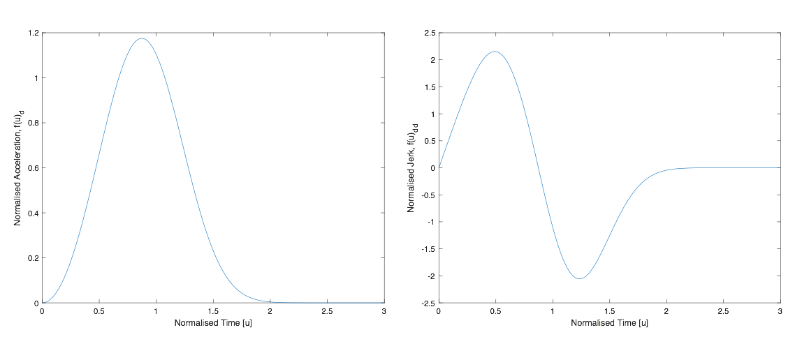
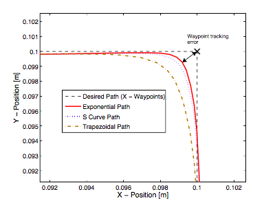
Exponential Method vs Trapezaoidal Method vs S-curve Method
Trajectory plan is an important step in precition motion. The S-curve method has a trapezoidal acceleration profile and a bounded jerk profile. The trapezoidal method has a rectangular acceleration and unbounded jerk profile, and the new-introduced exponential method has a near-sinusoidal jerk profile, as shown in the picture at the beginning. It was expected that the smoother the jerk profile is, the more accurate the path is. The repeated results also proved this hypothesis, as shown in the picture on the right.
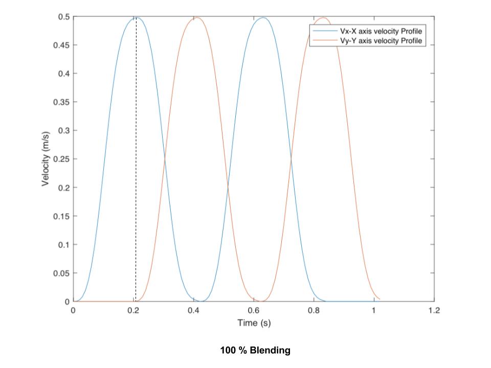
Blending Functionality
The blending functionality means, in a trajectory planning, each subsequent motion is started before the previous has reached its desired position. Otherwire, if each subsequent motion is started after the previous has reached its desired position, we say there is no blending, or there is 0% blending. The picture below shows an example of 100% blending.
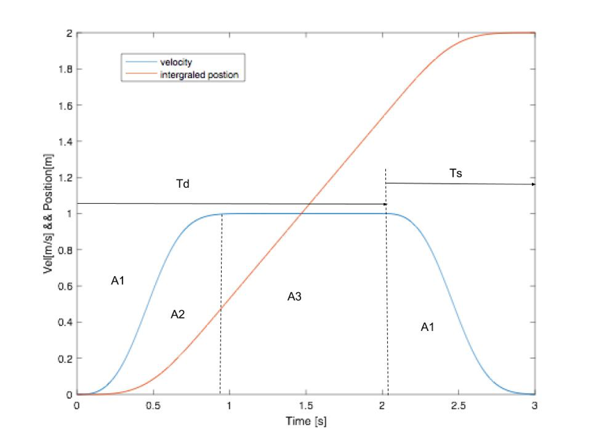
To further understanding the definition of blending functionality, let's introduce the exponential velocity profile first: As shown in the picture above, The x axis represents time in second, and the y axis represents velocity in m/s and position in meter.In the paper, an exponential velocity equation was given, and it is the blue line in the profile, then the velocity was integrated to find the instantaneous position of a path. In my integration, I applied the forward differentiation equation with the sampling time as 1 ms. For sequence of n motion, the total travel time Tt of a 0% blending is: Tt = ( X1 + X2 + ... + Xn ) / Vmax + n * Ts while the total travel time Tt of a 100% blending is: Tt = ( X1 + X2 + ... + Xn ) / Vmax + Ts
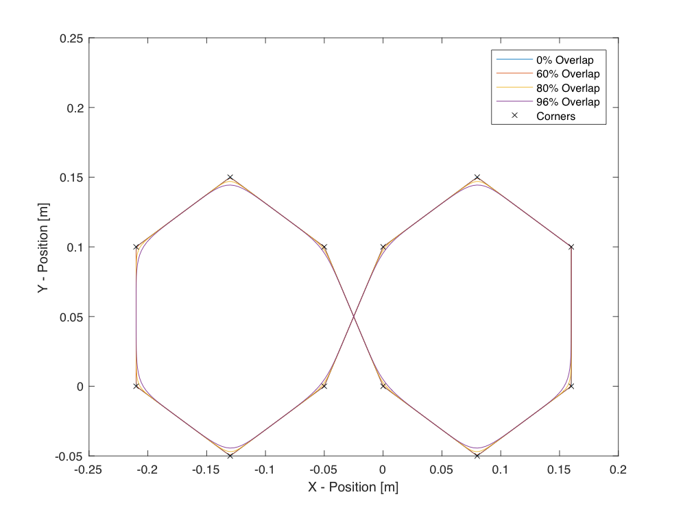
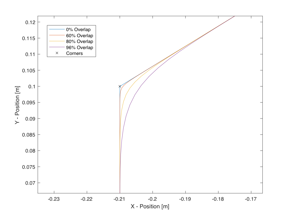
Based on the principles above, I reapeated the mathematical experiment in the paper: create a figure of eight path with various blend parameters. In my code, I did 0% overlap, 60% overlap, 80% overlap and 96% overlap for the same geometry. The result and the enlarged result are shown below:
As shown in the figure, the higher the parameter of blending, the less accurate of the path. Furhtermore, I calculated the motion durations with different percentage of overlap, and the result is tabulated below:
0% Overlap
60% Overlap
80% Overlap
96% Overlap
Tt (s)
5.0429
3.5655
3.0730
2.6790
As indicated in the table, the higher the parameter of blending, the less total travel time. Therefore, there is always a trade-off between the time optimal and accuracy.
In case for the further reference, below I attach the MATLAB code that I generated to repeat the blending results:
clear
clc

Ax=0.16; Ay=0.1;
Bx=0.08; By=0.15;
Cx=0; Cy=0.1;
Dx=-0.05; Dy=0;
Ex=-0.13; Ey=-0.05;
Fx=-0.21; Fy=0;
Gx=-0.21; Gy=0.1;
Hx=-0.13; Hy=0.15;
Ix=-0.05; Iy=0.1;
Jx=0; Jy=0;
Kx=0.08; Ky=-0.05;
Lx=0.16; Ly=0;

ABx=abs(Ax-Bx); ABy=abs(Ay-By);
BCx=abs(Bx-Cx); BCy=abs(By-Cy);
CDx=abs(Cx-Dx); CDy=abs(Cy-Dy);
DEx=abs(Dx-Ex); DEy=abs(Dy-Ey);
EFx=abs(Ex-Fx); EFy=abs(Ey-Fy);
FGx=abs(Fx-Gx); FGy=abs(Fy-Gy);
GHx=abs(Gx-Hx); GHy=abs(Gy-Hy);
HIx=abs(Hx-Ix); HIy=abs(Hy-Iy);
IJx=abs(Ix-Jx); IJy=abs(Iy-Jy);
JKx=abs(Jx-Kx); JKy=abs(Jy-Ky);
KLx=abs(Kx-Lx); KLy=abs(Ky-Ly);
LAx=abs(Lx-Ax); LAy=abs(Ly-Ay);

X=[ABx BCx CDx DEx EFx FGx GHx HIx IJx JKx KLx LAx];
Y=[ABy BCy CDy DEy EFy FGy GHy HIy IJy JKy KLy LAy];
XY=[sqrt(X.^2+Y.^2)]';

V_max=0.5; % m/s
A_max=5; % m/s^2
J_max=200; % m/s^3
d_t=0.01; % s
alpha=min(A_max/1.1754/V_max,sqrt(J_max/2.1524/V_max));
Ts=1.9045/alpha;

Td=XY./V_max;

% AB
t1=0:0.01:(Td(1)+Ts);
n1=numel(t1);
for k=1:n1
    ft_1=V_max.*(1-exp(-(alpha.*t1(k))^3));
    ft_2=V_max.*(1-exp(-(alpha.*(t1(k)-Td(1)))^3));
    if (t1(k)-Td(1))< 0
        H=0;
    else
        H=1;
    end
    v1(k)=ft_1-ft_2*H;
    v1x(k)=-v1(k).*cos(atan(0.5/0.8));
    v1y(k)=v1(k).*sin(atan(0.5/0.8));
end

% BC
t2=0:0.01:(Td(2)+Ts);
n2=numel(t2);
for k=1:n2
    ft_1=V_max.*(1-exp(-(alpha.*t2(k))^3));
    ft_2=V_max.*(1-exp(-(alpha.*(t2(k)-Td(2)))^3));
    if (t2(k)-Td(2))< 0
        H=0;
    else
        H=1;
    end
    v2(k)=ft_1-ft_2*H;
    v2x(k)=-v2(k).*cos(atan(0.5/0.8));
    v2y(k)=-v2(k).*sin(atan(0.5/0.8));
end

% CD
t3=0:0.01:(Td(3)+Ts);
n3=numel(t3);
for k=1:n3
    ft_1=V_max.*(1-exp(-(alpha.*t3(k))^3));
    ft_2=V_max.*(1-exp(-(alpha.*(t3(k)-Td(3)))^3));
    if (t3(k)-Td(3))< 0
        H=0;
    else
        H=1;
    end
    v3(k)=ft_1-ft_2*H;
    v3x(k)=-v3(k).*cos(atan(0.1/0.05));
    v3y(k)=-v3(k).*sin(atan(0.1/0.05));
end

% DE
t4=0:0.01:(Td(4)+Ts);
n4=numel(t4);
for k=1:n4
    ft_1=V_max.*(1-exp(-(alpha.*t4(k))^3));
    ft_2=V_max.*(1-exp(-(alpha.*(t4(k)-Td(4)))^3));
    if (t4(k)-Td(4))< 0
        H=0;
    else
        H=1;
    end
    v4(k)=ft_1-ft_2*H;
    v4x(k)=-v4(k).*cos(atan(0.05/0.08));
    v4y(k)=-v4(k).*sin(atan(0.05/0.08));
end

% EF
t5=0:0.01:(Td(5)+Ts);
n5=numel(t5);
for k=1:n2
    ft_1=V_max.*(1-exp(-(alpha.*t5(k))^3));
    ft_2=V_max.*(1-exp(-(alpha.*(t5(k)-Td(5)))^3));
    if (t5(k)-Td(5))< 0
        H=0;
    else
        H=1;
    end
    v5(k)=ft_1-ft_2*H;
    v5x(k)=-v5(k).*cos(atan(0.5/0.8));
    v5y(k)=v5(k).*sin(atan(0.5/0.8));
end

% FG
t6=0:0.01:(Td(6)+Ts);
n6=numel(t6);
for k=1:n6
    ft_1=V_max.*(1-exp(-(alpha.*t6(k))^3));
    ft_2=V_max.*(1-exp(-(alpha.*(t6(k)-Td(6)))^3));
    if (t6(k)-Td(6))< 0
        H=0;
    else
        H=1;
    end
    v6(k)=ft_1-ft_2*H;
    v6x(k)=v6(k).*0;
    v6y(k)=v6(k);
end

% GH
t7=0:0.01:(Td(7)+Ts);
n7=numel(t7);
for k=1:n7
    ft_1=V_max.*(1-exp(-(alpha.*t7(k))^3));
    ft_2=V_max.*(1-exp(-(alpha.*(t7(k)-Td(7)))^3));
    if (t7(k)-Td(7))< 0
        H=0;
    else
        H=1;
    end
    v7(k)=ft_1-ft_2*H;
    v7x(k)=v7(k).*cos(atan(0.5/0.8));
    v7y(k)=v7(k).*sin(atan(0.5/0.8));
end

% HI
t8=0:0.01:(Td(8)+Ts);
n8=numel(t8);
for k=1:n8
    ft_1=V_max.*(1-exp(-(alpha.*t8(k))^3));
    ft_2=V_max.*(1-exp(-(alpha.*(t8(k)-Td(8)))^3));
    if (t8(k)-Td(8))< 0
        H=0;
    else
        H=1;
    end
    v8(k)=ft_1-ft_2*H;
    v8x(k)=v8(k).*cos(atan(0.5/0.8));
    v8y(k)=-v8(k).*sin(atan(0.5/0.8));
end

% IJ
t9=0:0.01:(Td(9)+Ts);
n9=numel(t9);
for k=1:n9
    ft_1=V_max.*(1-exp(-(alpha.*t9(k))^3));
    ft_2=V_max.*(1-exp(-(alpha.*(t9(k)-Td(9)))^3));
    if (t9(k)-Td(9))< 0
        H=0;
    else
        H=1;
    end
    v9(k)=ft_1-ft_2*H;
    v9x(k)=v9(k).*cos(atan(0.1/0.05));
    v9y(k)=-v9(k).*sin(atan(0.1/0.05));
end

% JK
t10=0:0.01:(Td(10)+Ts);
n10=numel(t10);
for k=1:n10
    ft_1=V_max.*(1-exp(-(alpha.*t10(k))^3));
    ft_2=V_max.*(1-exp(-(alpha.*(t10(k)-Td(10)))^3));
    if (t10(k)-Td(10))< 0
        H=0;
    else
        H=1;
    end
    v10(k)=ft_1-ft_2*H;
    v10x(k)=v10(k).*cos(atan(0.5/0.8));
    v10y(k)=-v10(k).*sin(atan(0.5/0.8));
end

% KL
t11=0:0.01:(Td(11)+Ts);
n11=numel(t11);
for k=1:n11
    ft_1=V_max.*(1-exp(-(alpha.*t11(k))^3));
    ft_2=V_max.*(1-exp(-(alpha.*(t11(k)-Td(11)))^3));
    if (t11(k)-Td(11))< 0
        H=0;
    else
        H=1;
    end
    v11(k)=ft_1-ft_2*H;
    v11x(k)=v11(k).*cos(atan(0.5/0.8));
    v11y(k)=v11(k).*sin(atan(0.5/0.8));
end

% LA
t12=0:0.01:(Td(12)+Ts);
n12=numel(t12);
for k=1:n12
    ft_1=V_max.*(1-exp(-(alpha.*t12(k))^3));
    ft_2=V_max.*(1-exp(-(alpha.*(t12(k)-Td(12)))^3));
    if (t12(k)-Td(12))< 0
        H=0;
    else
        H=1;
    end
    v12(k)=ft_1-ft_2*H;
    v12x(k)=v12(k).*0;
    v12y(k)=v12(k);
end

%% 0% Overlap
T_zero=sum(Td)+12*Ts;
Vx_zero=[v1x v2x v3x v4x v5x v6x v7x v8x v9x v10x v11x v12x];
Vy_zero=[v1y v2y v3y v4y v5y v6y v7y v8y v9y v10y v11y v12y];
X_zero(1)=0.16;
Y_zero(1)=0.1;
for k=1:numel(Vx_zero)
    X_zero(k+1)=Vx_zero(k).*d_t+X_zero(k);
    Y_zero(k+1)=Vy_zero(k).*d_t+Y_zero(k);
end
x_zero=X_zero(1:k);
y_zero=Y_zero(1:k);
plot(x_zero,y_zero)
hold on;

%% 60% Overlap
T_sixty=T_zero-11*0.6*Ts;
q=int16(0.6*Ts/d_t);
Vx_sixty=[v1x(1:(n1-q)) v1x((n1-q+1):n1)+v2x(1:q) v2x((q+1):(n2-q)) v2x((n2-q+1):n2)+v3x(1:q) v3x((q+1):(n3-q)) v3x((n3-q+1):n3)+v4x(1:q) v4x((q+1):(n4-q)) v4x((n4-q+1):n4)+v5x(1:q) v5x((q+1):(n5-q)) v5x((n5-q+1):n5)+v6x(1:q) v6x((q+1):(n6-q)) v6x((n6-q+1):n6)+v7x(1:q) v7x((q+1):(n7-q)) v7x((n7-q+1):n7)+v8x(1:q) v8x((q+1):(n8-q)) v8x((n8-q+1):n8)+v9x(1:q) v9x((q+1):(n9-q)) v9x((n9-q+1):n9)+v10x(1:q) v10x((q+1):(n10-q)) v10x((n10-q+1):n10)+v11x(1:q) v11x((q+1):(n11-q)) v11x((n11-q+1):n11)+v12x(1:q) v12x((q+1):n12)];
Vy_sixty=[v1y(1:(n1-q)) v1y((n1-q+1):n1)+v2y(1:q) v2y((q+1):(n2-q)) v2y((n2-q+1):n2)+v3y(1:q) v3y((q+1):(n3-q)) v3y((n3-q+1):n3)+v4y(1:q) v4y((q+1):(n4-q)) v4y((n4-q+1):n4)+v5y(1:q) v5y((q+1):(n5-q)) v5y((n5-q+1):n5)+v6y(1:q) v6y((q+1):(n6-q)) v6y((n6-q+1):n6)+v7y(1:q) v7y((q+1):(n7-q)) v7y((n7-q+1):n7)+v8y(1:q) v8y((q+1):(n8-q)) v8y((n8-q+1):n8)+v9y(1:q) v9y((q+1):(n9-q)) v9y((n9-q+1):n9)+v10y(1:q) v10y((q+1):(n10-q)) v10y((n10-q+1):n10)+v11y(1:q) v11y((q+1):(n11-q)) v11y((n11-q+1):n11)+v12y(1:q) v12y((q+1):n12)];
X_sixty(1)=0.16;
Y_sixty(1)=0.1;
for k=1:numel(Vx_sixty)
    X_sixty(k+1)=Vx_sixty(k).*d_t+X_sixty(k);
    Y_sixty(k+1)=Vy_sixty(k).*d_t+Y_sixty(k);
end
x_sixty=X_sixty(1:k);
y_sixty=Y_sixty(1:k);
plot(x_sixty,y_sixty)
hold on;

%% 80% Overlap
T_eighty=T_zero-11*0.8*Ts;
q=int16(0.8*Ts/d_t);
Vx_eighty=[v1x(1:(n1-q)) v1x((n1-q+1):n1)+v2x(1:q) v2x((q+1):(n2-q)) v2x((n2-q+1):n2)+v3x(1:q) v3x((q+1):(n3-q)) v3x((n3-q+1):n3)+v4x(1:q) v4x((q+1):(n4-q)) v4x((n4-q+1):n4)+v5x(1:q) v5x((q+1):(n5-q)) v5x((n5-q+1):n5)+v6x(1:q) v6x((q+1):(n6-q)) v6x((n6-q+1):n6)+v7x(1:q) v7x((q+1):(n7-q)) v7x((n7-q+1):n7)+v8x(1:q) v8x((q+1):(n8-q)) v8x((n8-q+1):n8)+v9x(1:q) v9x((q+1):(n9-q)) v9x((n9-q+1):n9)+v10x(1:q) v10x((q+1):(n10-q)) v10x((n10-q+1):n10)+v11x(1:q) v11x((q+1):(n11-q)) v11x((n11-q+1):n11)+v12x(1:q) v12x((q+1):n12)];
Vy_eighty=[v1y(1:(n1-q)) v1y((n1-q+1):n1)+v2y(1:q) v2y((q+1):(n2-q)) v2y((n2-q+1):n2)+v3y(1:q) v3y((q+1):(n3-q)) v3y((n3-q+1):n3)+v4y(1:q) v4y((q+1):(n4-q)) v4y((n4-q+1):n4)+v5y(1:q) v5y((q+1):(n5-q)) v5y((n5-q+1):n5)+v6y(1:q) v6y((q+1):(n6-q)) v6y((n6-q+1):n6)+v7y(1:q) v7y((q+1):(n7-q)) v7y((n7-q+1):n7)+v8y(1:q) v8y((q+1):(n8-q)) v8y((n8-q+1):n8)+v9y(1:q) v9y((q+1):(n9-q)) v9y((n9-q+1):n9)+v10y(1:q) v10y((q+1):(n10-q)) v10y((n10-q+1):n10)+v11y(1:q) v11y((q+1):(n11-q)) v11y((n11-q+1):n11)+v12y(1:q) v12y((q+1):n12)];
X_eighty(1)=0.16;
Y_eighty(1)=0.1;
for k=1:numel(Vx_eighty)
    X_eighty(k+1)=Vx_eighty(k).*d_t+X_eighty(k);
    Y_eighty(k+1)=Vy_eighty(k).*d_t+Y_eighty(k);
end
x_eighty=X_eighty(1:k);
y_eighty=Y_eighty(1:k);
plot(x_eighty,y_eighty)
hold on;

%% 96% Overlap
T_hun=T_zero-11*0.96*Ts;
q=floor(Ts*0.96/d_t);
Vx_hun=[v1x(1:(n1-q)) v1x((n1-q+1):n1)+v2x(1:q) v2x((q+1):(n2-q)) v2x((n2-q+1):n2)+v3x(1:q) v3x((q+1):(n3-q)) v3x((n3-q+1):n3)+v4x(1:q) v4x((q+1):(n4-q)) v4x((n4-q+1):n4)+v5x(1:q) v5x((q+1):(n5-q)) v5x((n5-q+1):n5)+v6x(1:q) v6x((q+1):(n6-q)) v6x((n6-q+1):n6)+v7x(1:q) v7x((q+1):(n7-q)) v7x((n7-q+1):n7)+v8x(1:q) v8x((q+1):(n8-q)) v8x((n8-q+1):n8)+v9x(1:q) v9x((q+1):(n9-q)) v9x((n9-q+1):n9)+v10x(1:q) v10x((q+1):(n10-q)) v10x((n10-q+1):n10)+v11x(1:q) v11x((q+1):(n11-q)) v11x((n11-q+1):n11)+v12x(1:q) v12x((q+1):n12)];
Vy_hun=[v1y(1:(n1-q)) v1y((n1-q+1):n1)+v2y(1:q) v2y((q+1):(n2-q)) v2y((n2-q+1):n2)+v3y(1:q) v3y((q+1):(n3-q)) v3y((n3-q+1):n3)+v4y(1:q) v4y((q+1):(n4-q)) v4y((n4-q+1):n4)+v5y(1:q) v5y((q+1):(n5-q)) v5y((n5-q+1):n5)+v6y(1:q) v6y((q+1):(n6-q)) v6y((n6-q+1):n6)+v7y(1:q) v7y((q+1):(n7-q)) v7y((n7-q+1):n7)+v8y(1:q) v8y((q+1):(n8-q)) v8y((n8-q+1):n8)+v9y(1:q) v9y((q+1):(n9-q)) v9y((n9-q+1):n9)+v10y(1:q) v10y((q+1):(n10-q)) v10y((n10-q+1):n10)+v11y(1:q) v11y((q+1):(n11-q)) v11y((n11-q+1):n11)+v12y(1:q) v12y((q+1):n12)];
X_hun(1)=0.16;
Y_hun(1)=0.1;
for k=1:numel(Vy_hun)
    X_hun(k+1)=Vx_hun(k).*d_t+X_hun(k);
    Y_hun(k+1)=Vy_hun(k).*d_t+Y_hun(k);
end
x_hun=X_hun(1:k);
y_hun=Y_hun(1:k);
plot(x_hun,y_hun)
plot(0.16,0.1,'kx',0.08,0.15,'kx',0,0.1,'kx',-0.05,0,'kx',-0.13,-0.05,'kx',-0.21,0,'kx',-0.21,0.1,'kx',-0.13,0.15,'kx',-0.05,0.1,'kx',0,0,'kx',0.08,-0.05,'kx',0.16,0,'kx');
hold off;
xlim([-0.25 0.2])
ylim([-0.05 0.25])
xlabel('X - Position [m]');
ylabel('Y - Position [m]');
legend('0% Overlap','60% Overlap','80% Overlap','96% Overlap','Corners');
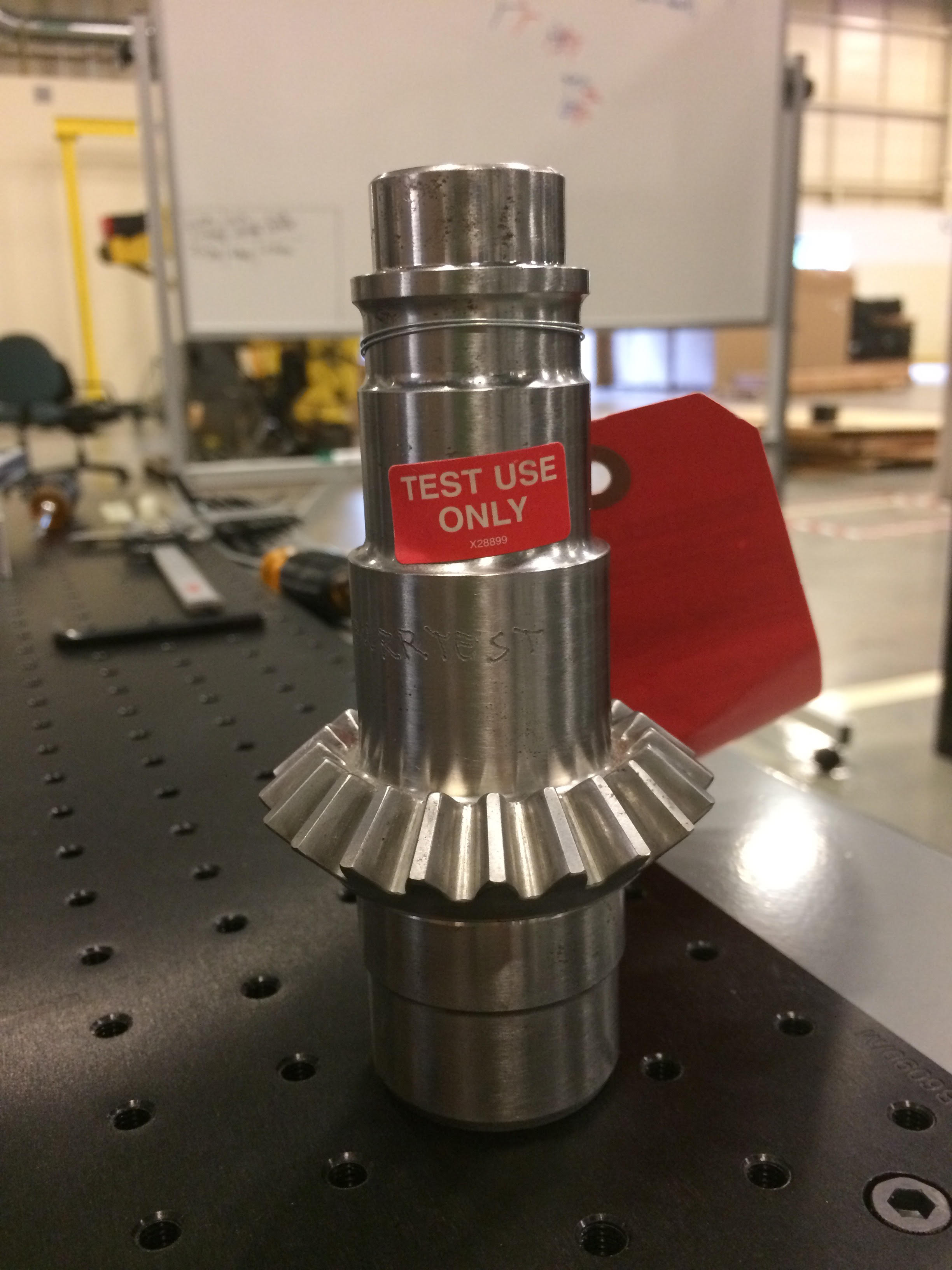 The purpose of this project is to deburr the Airplane Gear Teeth (shown in the pic. on the left) with the industrial robot. Even though the desired deburring path on the gear teeth is irregular, it is composed with basic configurations of circles and rectangles. Therefore, before actually deburring the gear teeth, we researched on deburring circular and rectangular aluminum blocks first to evaluate the methods and performances.
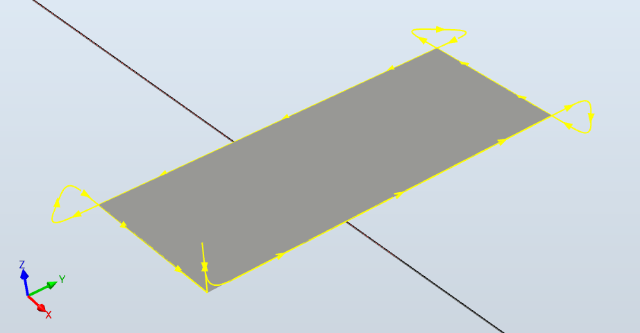 In this iteration for rectangle, besides changing the end effector tool orientation, I also edited the deburring path of the rectangle. As shown in the picture on the right, at each corner, I added an extra detour so that the robot did not have to stop to avoid the corner collisions.